Exploratory Data Analysis with CISSM Cyber Attacks Database - Part 2
Part 2 of 2
Introduction
In part 2 of our exploratory data analysis (EDA), a mission critical task underpinning the predominance of detection development and preparation for cybersecurity-centric machine learning, a remimder that there are a number of actions that analysts can take to better understand a particular data set and ready it for more robust utilization. That includes forecasting, which we will perform, again using the University of Maryland’s Center for International and Security Studies (CISSM) Cyber Attacks Database, an ideal candidate for experimental exploration. Per the dataset description, the database “brings together open-source information surrounding a range of publicly acknowledged cyber events on private and public organizations. Events from 2014 through present have been coded to standardize information on threat actor, threat actor country, motive, target, end effects, industry, and country of impact. Source links to the news source are also provided” (Harry & Gallagher, 2018).
We continue this exploratory data analytics journey with forecasting models and plots to show how you might predict future attack volumes.
Models
Next, we model the CISSM CAD data for time series forecasting with three well known methods selected for performance with the CISSM CAD dataset. These include naive, SES, and ARIMA.
Naive forecasting uses the most recent observation as the forecast for the next observation.
Simple exponential smoothing (SES) is the method of time series forecasting used with univariate data with no trend and no seasonal pattern.
Autoregressive integrated moving average, or ARIMA, is a statistical analysis model that uses time series data to either better understand the data set or to predict future trends.
Before we initiate the forecasts we use each of the methods to determine which one performs best. For brevity here, we’ll only run the models and plots on exploitative data, but the forecasts_CISSM.R script and the Jupyter/Colab notebook in the GitHub repo run all models and plots with disruptive and exploitative data. Note again that these are subsets of a much broader dataset represented by CISSM CAD. Explore further to your liking.
Important to the modeling that follows, note the evaluation metrics RMSE and MAE. Root Mean Squared Error (RMSE) and Mean Absolute Error (MAE) are used to evaluate regression models, tell us how accurate our predictions are, and the amount of deviation from actual values (Acharya, 2021). In essence, the lower the score, the better the performance.
> naive_model_exploitative <- naive(exploitative, h = 12)
> summary(naive_model_exploitative)

Forecast method: Naive method

Model Information:
Call: naive(y = exploitative, h = 12)

Residual sd: 20.5334

Error measures:
                      ME    RMSE      MAE  MPE MAPE      MASE       ACF1
Training set -0.06481481 20.5334 15.41667 -Inf  Inf 0.6228308 -0.3349566

Forecasts:
         Point Forecast      Lo 80     Hi 80      Lo 95     Hi 95
Feb 2023             23  -3.314606  49.31461  -17.24472  63.24472
Mar 2023             23 -14.214473  60.21447  -33.91463  79.91463
Apr 2023             23 -22.578235  68.57824  -46.70590  92.70590
May 2023             23 -29.629213  75.62921  -57.48944 103.48944
Jun 2023             23 -35.841249  81.84125  -66.98992 112.98992
Jul 2023             23 -41.457358  87.45736  -75.57902 121.57902
#snipped
The naive model yields an RMSE score of 20.5 and an MAE score 15.4.
> ses_model_exploitative <- ses(exploitative$Exploitative, h = 12) # RMSE = 18.8, MAE = 13.9
> summary(ses_model_exploitative)

Forecast method: Simple exponential smoothing

Model Information:
Simple exponential smoothing

Call:
 ses(y = exploitative$Exploitative, h = 12)

  Smoothing parameters:
    alpha = 0.529

  Initial states:
    l = 32.3171

  sigma:  19.0189

     AIC     AICc      BIC
1157.442 1157.671 1165.517

Error measures:
                    ME     RMSE      MAE  MPE MAPE      MASE       ACF1
Training set 0.2068036 18.84358 13.92841 -Inf  Inf 0.9034647 0.03522811

Forecasts:
    Point Forecast      Lo 80    Hi 80      Lo 95     Hi 95
110       44.24184 19.8681717 68.61551   6.965531  81.51815
111       44.24184 16.6677635 71.81592   2.070929  86.41275
112       44.24184 13.8020028 74.68168  -2.311874  90.79555
113       44.24184 11.1837445 77.29994  -6.316154  94.79983
114       44.24184  8.7581582 79.72552 -10.025768  98.50945
115       44.24184  6.4880896 81.99559 -13.497539 101.98122
#snipped
The SES model yields an RMSE score of 18.8 and an MAE score of 13.9.
> arima_model_exploitative <- auto.arima(exploitative)
> summary(arima_model_exploitative)
Series: exploitative
ARIMA(2,1,1)

Coefficients:
         ar1     ar2      ma1
      0.4744  0.1671  -0.9653
s.e.  0.1021  0.1007   0.0323

sigma^2 = 343.6:  log likelihood = -467.68
AIC=943.35   AICc=943.74   BIC=954.08

Training set error measures:
                   ME     RMSE     MAE  MPE MAPE      MASE        ACF1
Training set 2.152378 18.19375 13.5603 -Inf  Inf 0.5478338 -0.01933472
Finally, the ARIMA model yields an RMSE score of 18.2 and an MAE score of 13.6. Ultimately, by a small margin, the ARIMA model is most likely to provide the best forecast. Next, we forecast and plot the results. Given that ARIMA is most reliable under these circumstances, we’ll focus on visualizing ARIMA results; you can experiment with naive and SES plots on your own via the scripts or the notebook.
Forecasts & Plots
Generating a plot of AllEvents is as easy as:
autoplot(as.ts(AllEvents))
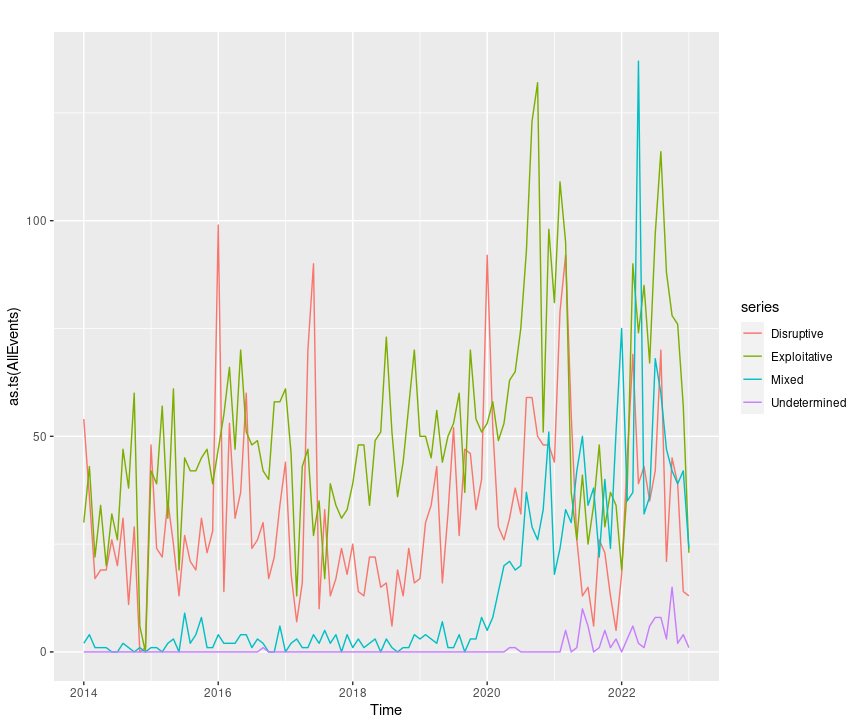
Figure 6: CISSM CAD AllEvents plot
This is just as easy with disruptive or exploitative events exclusively with the likes of autoplot(as.ts(disruptive)) or autoplot(as.ts(exploitative)).
To forecast the exploitative ARIMA model in an individual plot, utilize:
forecast(arima_model_exploitative) %>% autoplot()
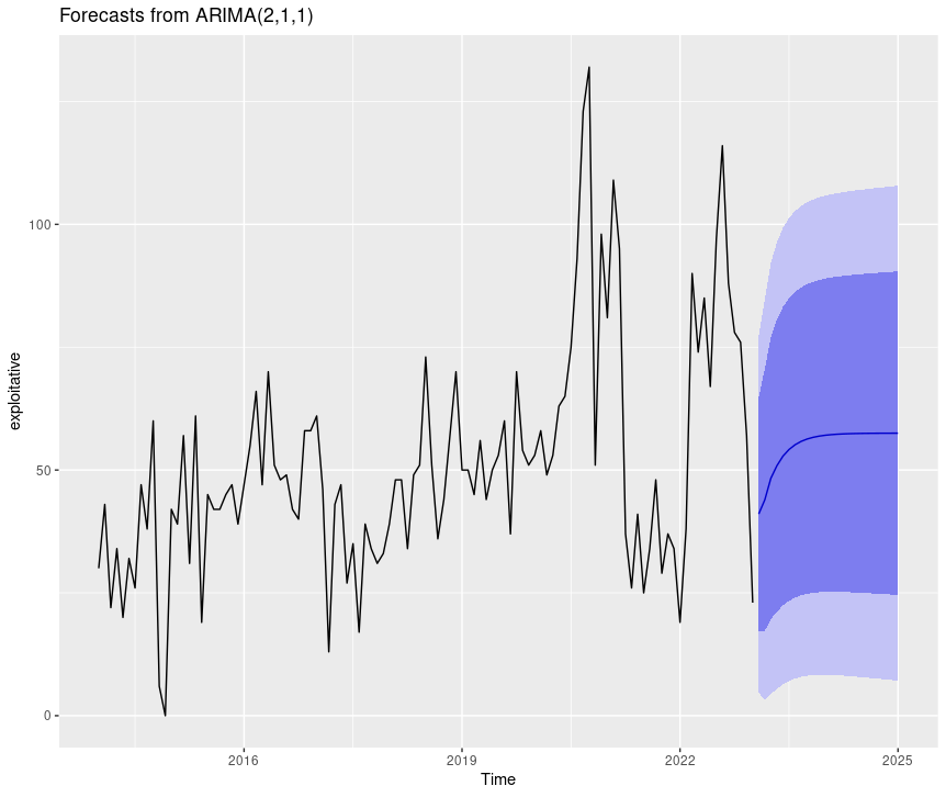
Figure 7: CISSM CAD exploitative events forecast plot
The light and dark areas correspond to the 95% and 80% confidence intervals (CI) respectively.
You can join multiple plots to compare outcomes side by side as follows.
naiveEXP = forecast(naive_model_exploitative) %>% autoplot()
sesEXP = forecast(ses_model_exploitative) %>% autoplot()
arimaEXP = forecast(arima_model_exploitative) %>% autoplot()

multi.pageEXP <- ggarrange(naiveEXP, sesEXP, arimaEXP, nrow = 3, ncol = 1)
multi.pageEXP
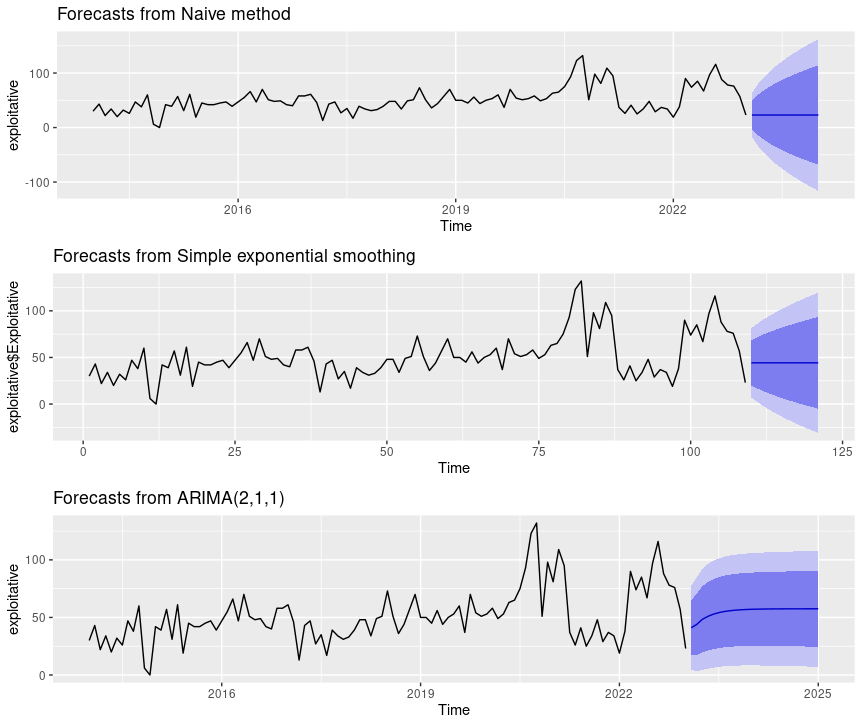
Figure 8: CISSM CAD exploitative events multi-model forecast plot
You may be wondering what ARIMA(2,1,1) refers to in our plots. A nonseasonal ARIMA model, which this is, is classified as an “ARIMA(p,d,q)” model, where: p is the number of autoregressive terms, d is the number of nonseasonal differences needed for stationarity, and q is the number of lagged forecast errors in the prediction equation. Therefore, in this case, (2,1,1) is p,d,q found by the auto.arima process indicating that we have two auto-regessive terms, one difference, and one moving average term in our series (Nau, 2020).
Conclusion
Hopefully, this effort has been useful and insightful for security analysts as well as fledgling data scientists in the security realm. It’s no surprise that I orient towards the practices of visualization; I have found all methods deployed here to be useful, effective, and durable for future use. It is my desire that you benefit similarly, and that this opens some doors for you, literally and figuratively.
Cheers…until next time.
Russ McRee | @holisticinfosec | infosec.exchange/@holisticinfosec | LinkedIn.com/in/russmcree


Comments