My Stack Simulator
The stack is a memory region where a program stores temporary data - like local variables and return addresses. Think of the stack as a pile of plates in your kitchen: you can only add a new plate to the top, and you can only take one away from the top too. Programs use this same "last in, first out" principle to keep track of what they're doing. Every time a function is called, the program pushes a new plate onto the stack containing things like local variables and the address to return to once the function finishes. When the function is done, that plate is popped off the top, and execution resumes exactly where it left off. This simple mechanism is what allows programs to call functions within functions within functions, and always find their way back - but it's also precisely why a stack that grows too large, or gets overwritten with unexpected data, becomes a favorite target for attackers looking to hijack a program's execution flow.
In the SANS class FOR610[1] (malware analysis), there is an introduction to assembly and, when students learn how functions work, they have to understand how the stack also works. If you’ve no prior experience, it could be a bit challenging. To help students to vizualise how the stack works, I created a “stack simulator” that allows to “see” what’s happening when code is executed.
How does it work?
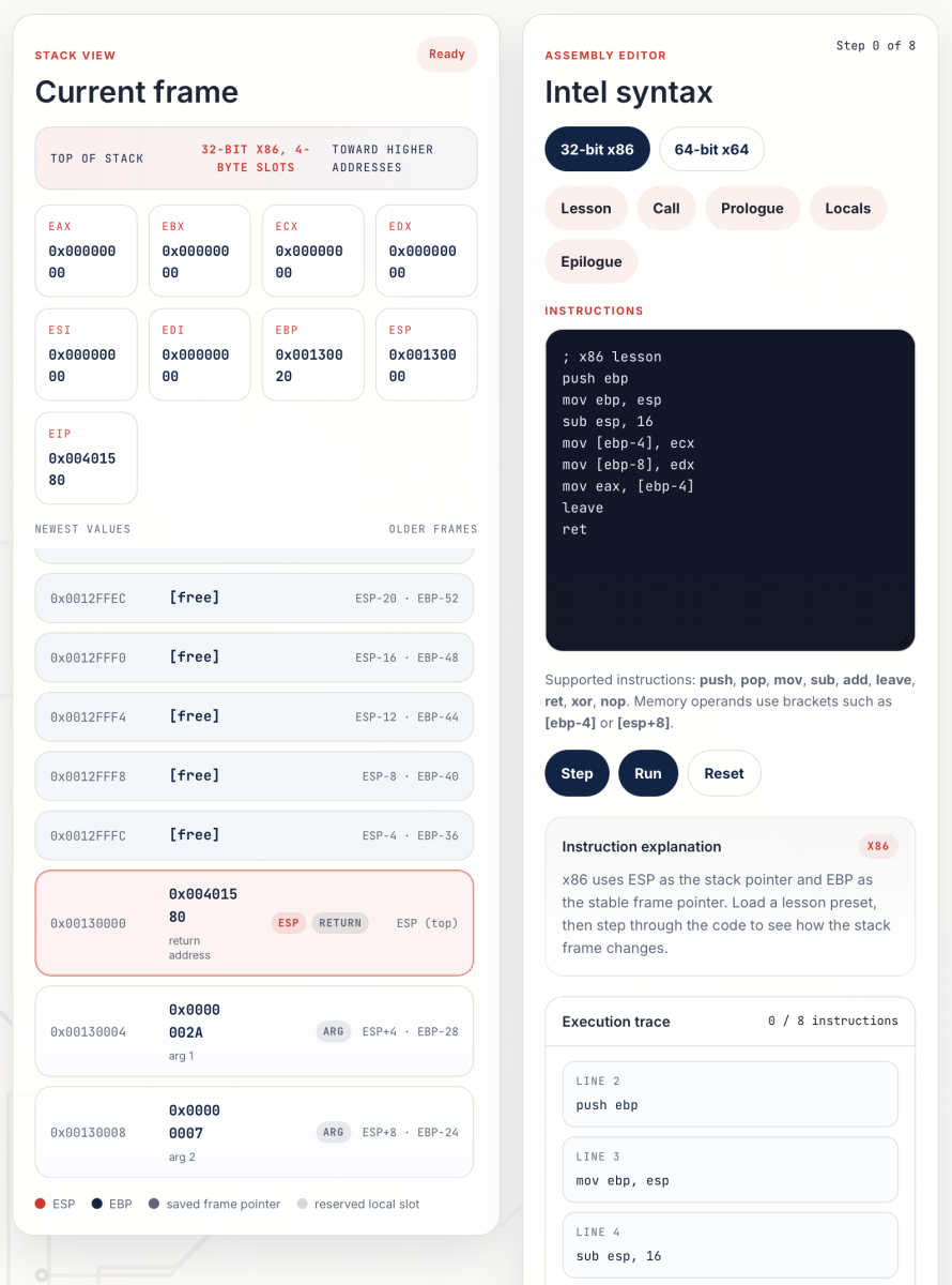
- Select the architecture (32-64 bits) in the assembly editor
- Select a predefined set of instructions (“lesson”, “call”, “prologue”, …).
- Click on “Step” to you can see the impact on the stack and registers (like in a debugger).
Note that you can modify the predefined ASM code and add your own instructions.
The stack simulator is available on my website[2].
If you’re interested in malware analysis, my next classes will be:
[1] https://www.sans.org/cyber-security-courses/reverse-engineering-malware-malware-analysis-tools-techniques
[2] https://xameco.be/stack-simulator.html
[3] https://www.sans.org/cyber-security-training-events/tokyo-autumn-2026
[4] https://www.sans.org/cyber-security-training-events/paris-november-2026
Xavier Mertens (@xme)
Xameco
Senior ISC Handler - Freelance Cyber Security Consultant
PGP Key


Comments